Comparing dynamic selection with Random Forest

In this example we use a pool of classifiers generated using the Random Forest method rather than Bagging. We also show how to change the size of the region of competence, used to estimate the local competence of the base classifiers.

This demonstrates that the library accepts any kind of base classifiers as long as they implement the predict and predict proba functions. Moreover, any ensemble generation method such as Boosting or Rotation Trees can be used to generate a pool containing diverse base classifiers. We also included the performance of the RandomForest classifier as a baseline comparison.

import matplotlib.pyplot as plt
from matplotlib.ticker import FuncFormatter
from matplotlib.cm import get_cmap
import numpy as np

# Example of a dcs techniques
from deslib.dcs.ola import OLA
from deslib.dcs.mcb import MCB
from deslib.des.des_p import DESP
from deslib.des.knora_u import KNORAU
from deslib.des.meta_des import METADES
from sklearn.datasets import load_breast_cancer
from sklearn.ensemble import RandomForestClassifier
from sklearn.model_selection import train_test_split

# Example of a des techniques
from deslib.des.knora_e import KNORAE

# Example of stacked model
from deslib.static.stacked import StackedClassifier
from sklearn.linear_model import LogisticRegression


rng = np.random.RandomState(42)

# Generate a classification dataset
data = load_breast_cancer()
X = data.data
y = data.target
# split the data into training and test data
X_train, X_test, y_train, y_test = train_test_split(X, y, test_size=0.25,
                                                    random_state=rng)
RF = RandomForestClassifier(random_state=rng)
RF.fit(X_train, y_train)

X_train, X_dsel, y_train, y_dsel = train_test_split(X_train, y_train,
                                                    test_size=0.50,
                                                    random_state=rng)

# Training a random forest to be used as the pool of classifiers.
# We set the maximum depth of the tree so that it
# can estimate probabilities
pool_classifiers = RandomForestClassifier(n_estimators=10, max_depth=5,
                                          random_state=rng)
pool_classifiers.fit(X_train, y_train)

stacked = StackedClassifier(pool_classifiers, LogisticRegression())
stacked.fit(X_dsel, y_dsel)

# Initialize a DS technique. Here we specify the size of
# the region of competence (5 neighbors)
knorau = KNORAU(pool_classifiers, random_state=rng)
kne = KNORAE(pool_classifiers, k=5, random_state=rng)
desp = DESP(pool_classifiers, k=5, random_state=rng)
ola = OLA(pool_classifiers, k=5, random_state=rng)
mcb = MCB(pool_classifiers, k=5, random_state=rng)
meta = METADES(pool_classifiers, k=5, random_state=rng)

# Fit the DS techniques
knorau.fit(X_dsel, y_dsel)
kne.fit(X_dsel, y_dsel)
desp.fit(X_dsel, y_dsel)
meta.fit(X_dsel, y_dsel)
ola.fit(X_dsel, y_dsel)
mcb.fit(X_dsel, y_dsel)

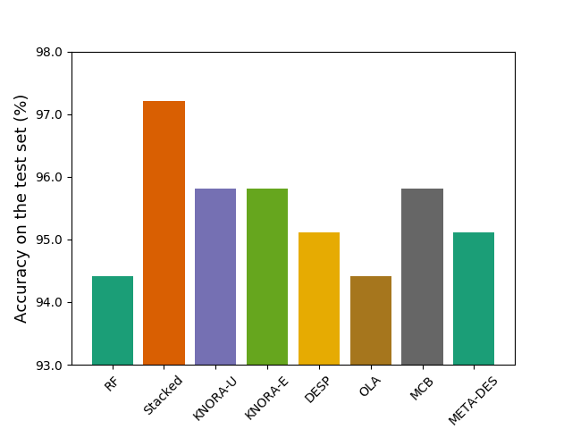
Plotting the results

Let’s now evaluate the methods on the test set.

rf_score = RF.score(X_test, y_test)
stacked_score = stacked.score(X_test, y_test)
knorau_score = knorau.score(X_test, y_test)
kne_score = kne.score(X_test, y_test)
desp_score = desp.score(X_test, y_test)
ola_score = ola.score(X_test, y_test)
mcb_score = mcb.score(X_test, y_test)
meta_score = meta.score(X_test, y_test)
print('Classification accuracy RF: ', rf_score)
print('Classification accuracy Stacked: ', stacked_score)
print('Evaluating DS techniques:')
print('Classification accuracy KNORA-U: ', knorau_score)
print('Classification accuracy KNORA-E: ', kne_score)
print('Classification accuracy DESP: ', desp_score)
print('Classification accuracy OLA: ', ola_score)
print('Classification accuracy MCB: ', mcb_score)
print('Classification accuracy META-DES: ', meta_score)

cmap = get_cmap('Dark2')
colors = [cmap(i) for i in np.linspace(0, 1, 7)]
labels = ['RF', 'Stacked', 'KNORA-U', 'KNORA-E', 'DESP', 'OLA', 'MCB',
          'META-DES']

fig, ax = plt.subplots()
pct_formatter = FuncFormatter(lambda x, pos: '{:.1f}'.format(x * 100))
ax.bar(np.arange(8),
       [rf_score, stacked_score, knorau_score, kne_score, desp_score,
        ola_score, mcb_score, meta_score],
       color=colors,
       tick_label=labels)
ax.set_ylim(0.93, 0.98)
ax.set_xlabel('Method', fontsize=13)
ax.set_ylabel('Accuracy on the test set (%)', fontsize=13)
ax.yaxis.set_major_formatter(pct_formatter)
for tick in ax.get_xticklabels():
    tick.set_rotation(45)
plt.subplots_adjust(bottom=0.15)
plt.show()

Out:

Classification accuracy RF:  0.9440559440559441
Classification accuracy Stacked:  0.972027972027972
Evaluating DS techniques:
Classification accuracy KNORA-U:  0.958041958041958
Classification accuracy KNORA-E:  0.958041958041958
Classification accuracy DESP:  0.951048951048951
Classification accuracy OLA:  0.9440559440559441
Classification accuracy MCB:  0.958041958041958
Classification accuracy META-DES:  0.951048951048951

Total running time of the script: ( 0 minutes 1.062 seconds)