Using the Dynamic Frienemy Pruning (DFP)

In this example we show how to apply the dynamic frienemy pruning (DFP) to different dynamic selection techniques.

The DFP method is an online pruning model which analyzes the region of competence to know if it is composed of samples from different classes (indecision region). Then, it remove the base classifiers that do not correctly classifies at least a pair of samples coming from different classes, i.e., the base classifiers that cannot separate the classes in the local region. More information on this method can be found in refs [1] and [2].

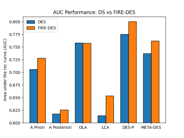
DES techniques using the DFP algorithm are called FIRE-DES (Frienemy Indecision REgion Dynamic Ensemble Selection). The FIRE-DES is shown to significantly improve the performance of several dynamic selection algorithms when dealing with imbalanced classification problems as it avoids the classifiers that are biased towards the majority class in predicting the label for the query.

References

[1] Oliveira, D.V.R., Cavalcanti, G.D.C. and Sabourin, R., “Online Pruning of Base Classifiers for Dynamic Ensemble Selection”, Pattern Recognition, vol. 72, 2017, pp 44-58.

[2] Cruz, R.M.O., Oliveira, D.V.R., Cavalcanti, G.D.C. and Sabourin, R., “FIRE-DES++: Enhanced online pruning of base classifiers for dynamic ensemble selection”., Pattern Recognition, vol. 85, 2019, pp 149-160.

import numpy as np
from sklearn.datasets import make_classification
from sklearn.ensemble import RandomForestClassifier
from sklearn.model_selection import train_test_split
from sklearn.metrics import roc_auc_score
import matplotlib.pyplot as plt
from deslib.dcs import APosteriori
from deslib.dcs import APriori
from deslib.dcs import LCA
from deslib.dcs import OLA
from deslib.des import DESP
from deslib.des import METADES

rng = np.random.RandomState(654321)

# Generate an imbalanced classification dataset
X, y = make_classification(n_classes=2, n_samples=2000, weights=[0.05, 0.95],
                           random_state=rng)
# split the data into training and test data
X_train, X_test, y_train, y_test = train_test_split(X, y, test_size=0.33,
                                                    random_state=rng)

# Split the data into training and DSEL for DS techniques
X_train, X_dsel, y_train, y_dsel = train_test_split(X_train, y_train,
                                                    test_size=0.5,
                                                    random_state=rng)
# Considering a pool composed of 10 base classifiers
pool_classifiers = RandomForestClassifier(n_estimators=10, random_state=rng,
                                          max_depth=10)
pool_classifiers.fit(X_train, y_train)

ds_names = ['A Priori', 'A Posteriori', 'OLA', 'LCA', 'DES-P', 'META-DES']

# DS techniques without DFP
apriori = APriori(pool_classifiers, random_state=rng)
aposteriori = APosteriori(pool_classifiers, random_state=rng)
ola = OLA(pool_classifiers)
lca = LCA(pool_classifiers)
desp = DESP(pool_classifiers)
meta = METADES(pool_classifiers)

# FIRE-DS techniques (with DFP)
fire_apriori = APriori(pool_classifiers, DFP=True, random_state=rng)
fire_aposteriori = APosteriori(pool_classifiers, DFP=True, random_state=rng)
fire_ola = OLA(pool_classifiers, DFP=True)
fire_lca = LCA(pool_classifiers, DFP=True)
fire_desp = DESP(pool_classifiers, DFP=True)
fire_meta = METADES(pool_classifiers, DFP=True)

list_ds = [apriori, aposteriori, ola, lca, desp, meta]
list_fire_ds = [fire_apriori, fire_aposteriori, fire_ola,
                fire_lca, fire_desp, fire_meta]

scores_ds = []
for ds in list_ds:
    ds.fit(X_dsel, y_dsel)
    scores_ds.append(roc_auc_score(y_test, ds.predict(X_test)))

scores_fire_ds = []
for fire_ds in list_fire_ds:
    fire_ds.fit(X_dsel, y_dsel)
    scores_fire_ds.append(roc_auc_score(y_test, fire_ds.predict(X_test)))

Comparing DS techniques with FIRE-DES techniques

Let’s now evaluate the DES methods on the test set. Since we are dealing with imbalanced data, we use the area under the roc curve (AUC) as performance metric instead of classification accuracy. The AUC can be easily calculated using the sklearn.metrics.roc_auc_score function from scikit-learn.

width = 0.35
ind = np.arange(len(ds_names))
plt.bar(ind, scores_ds, width, label='DES', edgecolor='k')
plt.bar(ind + width, scores_fire_ds, width, label='FIRE-DES', edgecolor='k')

plt.ylabel('Area under the roc curve (AUC)')
plt.title('AUC Performance: DS vs FIRE-DES')
plt.ylim((0.60, 0.81))
plt.xticks(ind + width / 2, ds_names)
plt.legend(loc='best')
plt.show()