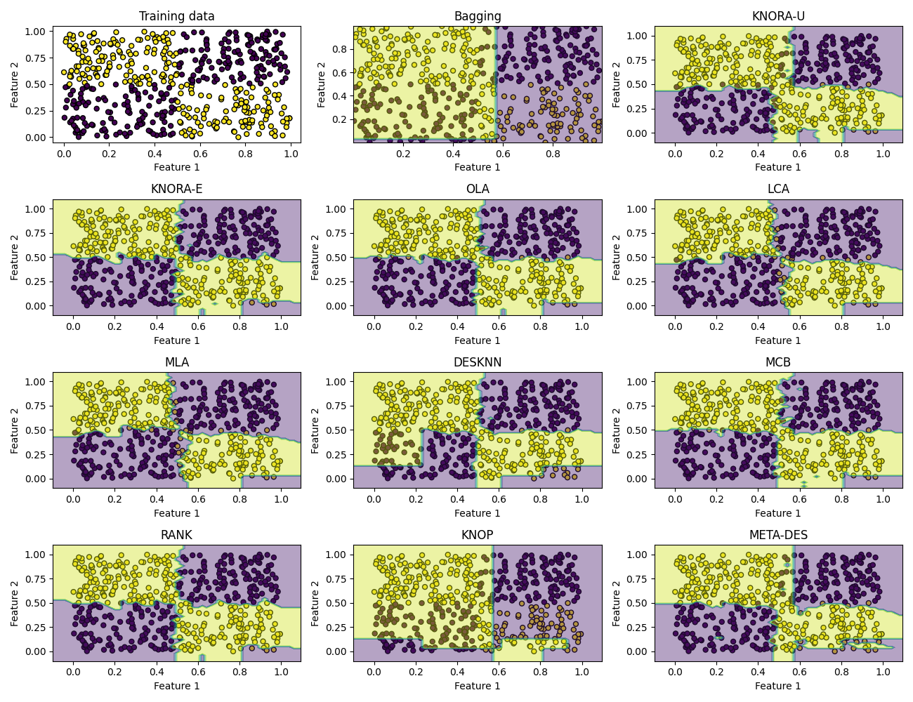
Dynamic selection with linear classifiers: XOR example

This example shows that DS can deal with non-linear problem (XOR) using a combination of a few linear base classifiers.

• 10 dynamic selection methods (5 DES and 5 DCS) are evaluated with a pool composed of Decision stumps.
• Since we use Bagging to generate the base classifiers, we also included its performance as a baseline comparison.

import matplotlib.pyplot as plt
import numpy as np
from sklearn.ensemble import BaggingClassifier
from sklearn.model_selection import train_test_split
from sklearn.tree import DecisionTreeClassifier

from deslib.dcs import LCA
from deslib.dcs import MLA
from deslib.dcs import OLA
from deslib.dcs import MCB
from deslib.dcs import Rank

from deslib.des import DESKNN
from deslib.des import KNORAE
from deslib.des import KNORAU
from deslib.des import KNOP
from deslib.des import METADES
from deslib.util.datasets import make_xor

Defining helper functions to facilitate plotting the decision boundaries:

def plot_classifier_decision(ax, clf, X, mode='line', **params):

    xx, yy = make_grid(X[:, 0], X[:, 1])

    Z = clf.predict(np.c_[xx.ravel(), yy.ravel()])
    Z = Z.reshape(xx.shape)
    if mode == 'line':
        ax.contour(xx, yy, Z, **params)
    else:
        ax.contourf(xx, yy, Z, **params)
    ax.set_xlim((np.min(X[:, 0]), np.max(X[:, 0])))
    ax.set_ylim((np.min(X[:, 1]), np.max(X[:, 0])))


def plot_dataset(X, y, ax=None, title=None, **params):

    if ax is None:
        ax = plt.gca()
    ax.scatter(X[:, 0], X[:, 1], marker='o', c=y, s=25,
               edgecolor='k', **params)
    ax.set_xlabel('Feature 1')
    ax.set_ylabel('Feature 2')
    if title is not None:
        ax.set_title(title)
    return ax


def make_grid(x, y, h=.02):

    x_min, x_max = x.min() - 1, x.max() + 1
    y_min, y_max = y.min() - 1, y.max() + 1
    xx, yy = np.meshgrid(np.arange(x_min, x_max, h),
                         np.arange(y_min, y_max, h))
    return xx, yy


# Prepare the DS techniques. Changing k value to 5.
def initialize_ds(pool_classifiers, X, y, k=5):
    knorau = KNORAU(pool_classifiers, k=k)
    kne = KNORAE(pool_classifiers, k=k)
    desknn = DESKNN(pool_classifiers, k=k)
    ola = OLA(pool_classifiers, k=k)
    lca = LCA(pool_classifiers, k=k)
    mla = MLA(pool_classifiers, k=k)
    mcb = MCB(pool_classifiers, k=k)
    rank = Rank(pool_classifiers, k=k)
    knop = KNOP(pool_classifiers, k=k)
    meta = METADES(pool_classifiers, k=k)

    list_ds = [knorau, kne, ola, lca, mla, desknn, mcb, rank, knop, meta]
    names = ['KNORA-U', 'KNORA-E', 'OLA', 'LCA', 'MLA', 'DESKNN', 'MCB',
             'RANK', 'KNOP', 'META-DES']
    # fit the ds techniques
    for ds in list_ds:
        ds.fit(X, y)

    return list_ds, names

Generating the dataset and training the pool of classifiers.

rng = np.random.RandomState(1234)
X, y = make_xor(1000, random_state=rng)
X_train, X_test, y_train, y_test = train_test_split(X, y, test_size=0.5,
                                                    random_state=rng)
X_DSEL, X_test, y_DSEL, y_test = train_test_split(X_train, y_train,
                                                  test_size=0.5,
                                                  random_state=rng)

pool_classifiers = BaggingClassifier(DecisionTreeClassifier(max_depth=1),
                                     n_estimators=10,
                                     random_state=rng)
pool_classifiers.fit(X_train, y_train)

Out:

BaggingClassifier(base_estimator=DecisionTreeClassifier(max_depth=1),
                  random_state=RandomState(MT19937) at 0x7F883E86F780)

Merging training and validation data to compose DSEL

In this example merge the training data with the validation, to create a DSEL having more examples for the competence estimation. Using the training data for dynamic selection can be beneficial when dealing with small sample size datasets. However, in this case we need to have a pool composed of weak classifier so that the base classifiers are not able to memorize the training data (overfit).

X_DSEL = np.vstack((X_DSEL, X_train))
y_DSEL = np.hstack((y_DSEL, y_train))
list_ds, names = initialize_ds(pool_classifiers, X_DSEL, y_DSEL, k=7)

fig, sub = plt.subplots(4, 3, figsize=(13, 10))
plt.subplots_adjust(wspace=0.4, hspace=0.4)

ax_data = sub.flatten()[0]
ax_bagging = sub.flatten()[1]
plot_dataset(X_train, y_train, ax=ax_data, title="Training data")

plot_dataset(X_train, y_train, ax=ax_bagging)
plot_classifier_decision(ax_bagging, pool_classifiers,
                         X_train, mode='filled', alpha=0.4)
ax_bagging.set_title("Bagging")

# Plotting the decision border of the DS methods
for ds, name, ax in zip(list_ds, names, sub.flatten()[2:]):
    plot_dataset(X_train, y_train, ax=ax)
    plot_classifier_decision(ax, ds, X_train, mode='filled', alpha=0.4)
    ax.set_xlim((np.min(X_train[:, 0]) - 0.1, np.max(X_train[:, 0] + 0.1)))
    ax.set_ylim((np.min(X_train[:, 1]) - 0.1, np.max(X_train[:, 1] + 0.1)))
    ax.set_title(name)
plt.show()
plt.tight_layout()

Evaluation on the test set

Finally, let’s evaluate the classification accuracy of DS techniques and Bagging on the test set:

for ds, name in zip(list_ds, names):
    print('Accuracy ' + name + ': ' + str(ds.score(X_test, y_test)))
print('Accuracy Bagging: ' + str(pool_classifiers.score(X_test, y_test)))

Out:

Accuracy KNORA-U: 0.92
Accuracy KNORA-E: 0.992
Accuracy OLA: 0.976
Accuracy LCA: 0.944
Accuracy MLA: 0.944
Accuracy DESKNN: 0.908
Accuracy MCB: 0.968
Accuracy RANK: 0.992
Accuracy KNOP: 0.636
Accuracy META-DES: 0.928
Accuracy Bagging: 0.584